User Tutorial
In the IPython Notebook, the ipymd package must first be imported:
import ipymd
print ipymd.version()
0.4.2
Basic Atom Creation and Visualisation
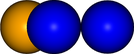
The input for a basic atomic visualisation, is a pandas Dataframe that specifies the coordinates, size and color of each atom in the following manner:
import pandas as pd
df = pd.DataFrame(
        [[2,3,4,1,[0, 0, 255],1],
         [1,3,3,1,'orange',1],
         [4,3,1,1,'blue',1]],
        columns=['x','y','z','radius','color','transparency'])
Distances are measured in Angstroms, and colors can be defined in
[r,g,b] format (0 to 255) or as a string defined in
available_colors.
print(ipymd.available_colors()['reds'])
['light_salmon', 'salmon', 'dark_salmon', 'light_coral', 'indian_red', 'crimson', 'fire_brick', 'dark_red', 'red']
The Visualise_Sim class can then be used to setup a visualisation,
which is returned in the form of a PIL image.
vis = ipymd.visualise_sim.Visualise_Sim()
vis.add_atoms(df)
img1 = vis.get_image(size=400,quality=5)
img1

To convert this into an image viewable in IPython, simply parse it to
the visualise function.
vis.visualise(img1)
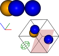
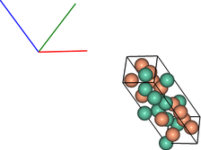
Extending this basic procedure, additional objects can be added to the visualisation, the viewpoint can be rotated and multiple images can be output at once, as shown in the following example:
vis.add_axes(length=0.2, offset=(-0.3,0))
vis.add_box([5,0,0],[0,5,0],[0,0,5])
vis.add_plane([[5,0,0],[0,5,2]],alpha=0.3)
vis.add_hexagon([[1,0,0],[0,0,.5]],[0,0,2],color='green')

img_ex1 = vis.get_image(xrot=45, yrot=45)
#img2 = vis.draw_colorlegend(img2,1,2)
vis.visualise([img1,img_ex1])
Atom Creation From Other Sources
The ipymd.data_input module includes a number of classes to automate
the intial creation of the atoms Dataframe, from various sources.
All classes will return a sub-class of DataInput, that requires the
setup_data method to be run first, and then the get_atoms method
returns the atoms Dataframe and the get_meta_data method returns a
Pandas Series (which includes the vertexes and origin of the simulation
box).
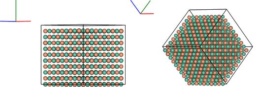
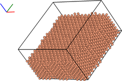
Crystal Parameters
This class allows atoms to be created in ordered crystal, as defined by their space group and crystal parameters:
data = ipymd.data_input.crystal.Crystal()
data.setup_data(
    [[0.0, 0.0, 0.0], [0.5, 0.5, 0.5]], ['Na', 'Cl'],
    225, cellpar=[5.4, 5.4, 5.4, 90, 90, 90],
    repetitions=[5, 5, 5])
meta = data.get_meta_data()
print meta
atoms_df = data.get_atom_data()
atoms_df.head(2)
origin                                 (0.0, 0.0, 0.0)
a                                     (27.0, 0.0, 0.0)
b                       (1.65327317885e-15, 27.0, 0.0)
c         (1.65327317885e-15, 1.65327317885e-15, 27.0)
dtype: object
| id | type | x | y | z | transparency | color | radius | |
|---|---|---|---|---|---|---|---|---|
| 0 | 1 | Na | 0.000000e+00 | 0.0 | 0.0 | 1.0 | light_salmon | 1.0 |
| 1 | 2 | Na | 3.306546e-16 | 2.7 | 2.7 | 1.0 | light_salmon | 1.0 |
vis2 = ipymd.visualise_sim.Visualise_Sim()
vis2.add_axes()
vis2.add_box(meta.a,meta.b,meta.c, meta.origin)
vis2.add_atoms(atoms_df)
images = [vis2.get_image(xrot=xrot,yrot=45) for xrot in [0,45]]
vis2.visualise(images, columns=2)
A dataframe is available which lists the alternative names for each space group:
df = ipymd.data_input.crystal.get_spacegroup_df()
df.loc[[1,194,225]]
| System_type | Point group | Short_name | Full_name | Schoenflies | Fedorov | Shubnikov | Fibrifold | |
|---|---|---|---|---|---|---|---|---|
| Number | ||||||||
| 1 | triclinic | 1 | P1 | P 1 | $C_1^1$ | 1s | $(a/b/c)\cdot 1$ | - |
| 194 | hexagonal | 6/m 2/m 2/m | P63/mmc | P 63/m 2/m 2/c | $D_{6h}^4$ | 88a | $(c:(a/a))\cdot m:6_3\cdot m$ | - |
| 225 | cubic | 4/m 3 2/m | Fm3m | F 4/m 3 2/m | $O_h^5$ | 73s | $\left ( \frac{a+c}{2}/\frac{b+c}{2}/\frac{a+b... | $2^{-}:2$ |
Crystallographic Information Files
.cif files are a common means to store crystallographic data and can be loaded as follows:
cif_path = ipymd.get_data_path('example_crystal.cif')
data = ipymd.data_input.cif.CIF()
data.setup_data(cif_path)
meta = data.get_meta_data()
vis = ipymd.visualise_sim.Visualise_Sim()
vis.basic_vis(data.get_atom_data(), data.get_meta_data(),
              xrot=45,yrot=45)
NB: at present, fractional occupancies of lattice sites are returned in the atom Dataframe, but cannot be visualised as such. It is intended that eventually occupancy will be visualised by partial spheres.
data.get_atom_data().head(1)
| type | x | y | z | occupancy | transparency | color | radius | |
|---|---|---|---|---|---|---|---|---|
| 0 | Fe | 4.363536 | 2.40065 | 22.642804 | 1.0 | 1.0 | light_salmon | 1.0 |
Lammps Input Data
The input data for LAMMPS simulations (supplied to read_data) can be
input. Note that the get_atom_data method requires that the
atom_style is defined, in order to define what each data column refers
to.
lammps_path = ipymd.get_data_path('lammps_input.data')
data = ipymd.data_input.lammps.LAMMPS_Input()
data.setup_data(lammps_path,atom_style='charge')
vis = ipymd.visualise_sim.Visualise_Sim()
vis.basic_vis(data.get_atom_data(), data.get_meta_data(),
              xrot=45,yrot=45)
Lammps Output Data
Output data can be read in the form of a single file or, it is advisable
for efficiency, that a single file is output for each timestep, where
* is used to define the variable section of the filename. The
get_atoms and get_simulation_box methods now take a variable to
define which configuration is returned.
lammps_path = ipymd.get_data_path('atom_onefile.dump')
data = ipymd.data_input.lammps.LAMMPS_Output()
data.setup_data(lammps_path)
print data.count_configs()

vis = ipymd.visualise_sim.Visualise_Sim()
vis.basic_vis(data.get_atom_data(99), data.get_meta_data(99),
              spheres=True,xrot=45,yrot=45,quality=5)
99
lammps_path = ipymd.get_data_path(['atom_dump','atoms_*.dump'])
data = ipymd.data_input.lammps.LAMMPS_Output()
data.setup_data(lammps_path)
print data.count_configs()

vis = ipymd.visualise_sim.Visualise_Sim()
vis.basic_vis(data.get_atom_data(99), data.get_meta_data(99),
              spheres=False,xrot=90,yrot=0)
99
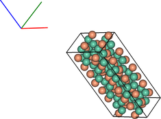
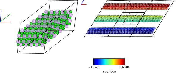
Atom Manipulation
The atoms Dataframe is already very easy to manipulate using the
standard pandas methods. But an
Atom_Manipulation class has also been created to carry out standard
atom manipulations, such as setting variables dependant on atom type or
altering the geometry, as shown in this example:
data = ipymd.data_input.crystal.Crystal()
data.setup_data(
    [[0.0, 0.0, 0.0], [0.5, 0.5, 0.5]], ['Na', 'Cl'],
    225, cellpar=[5.4, 5.4, 5.4,60,60,60],
    repetitions=[5, 5, 5])
meta = data.get_meta_data()

manipulate_atoms = ipymd.atom_manipulation.Atom_Manipulation

new_df = manipulate_atoms(data.get_atom_data(), data.get_meta_data(),undos=2)

new_df.apply_map({'Na':1.5, 'Cl':1},'radius')
new_df.apply_map('color','color',default='grey')
new_df.change_type_variable('Na', 'transparency', 0.5)
new_df.slice_fraction(cmin=0.3, cmax=0.7,update_uc=False)

vis2 = ipymd.visualise_sim.Visualise_Sim()
vis2.add_box(*new_df.meta[['a','b','c','origin']])
vis2.add_axes([meta.a,meta.b,meta.c],offset=(-1.3,-0.7))
vis2.add_atoms(new_df.df, spheres=True)

img1 = vis2.get_image(xrot=45,yrot=45)

vis2.remove_atoms()
new_df.repeat_cell((-1,1),(-1,1),(-1,1))
new_df.color_by_variable('z')
vis2.add_atoms(new_df.df, spheres=True)
vis2.add_box(*new_df.meta[['a','b','c','origin']])
img2 = vis2.get_image(xrot=90,yrot=0)
img3 = ipymd.plotting.create_colormap_image(new_df.df.z.min(), new_df.df.z.max(),
                                            horizontal=True,title='z position',size=150)

vis2.visualise([img1,img2, (280,1), img3], columns=2)
NB: default atom variables (such as color and radii can be set using the
apply_map method and any column name from those given in
ipymd.shared.atom_data():
ipymd.shared.atom_data().head(1)
| Num | ARENeg | RCov | RBO | RVdW | MaxBnd | Mass | ElNeg | Ionization | ElAffinity | Name | color_chemlab | color_chemlab_light | color | |
|---|---|---|---|---|---|---|---|---|---|---|---|---|---|---|
| Symb | ||||||||||||||
| H | 1 | 2.2 | 0.31 | 0.31 | 1.1 | 1 | 1.00794 | 2.2 | 13.5984 | 0.754204 | Hydrogen | white | snow | (191, 191, 191) |
Geometric Analysis
Given the simple and flexible form of the atomic data and visualisation,
it is now easier to add more complex geometric analysis. These analyses
are being contained in the atom_analysis package, and some initial
examples are detailed below. Functions in the
atom_analysis.nearest_neighbour package are based on the
scipy.spatial.cKDTree algorithm for identifying nearest neighbours.
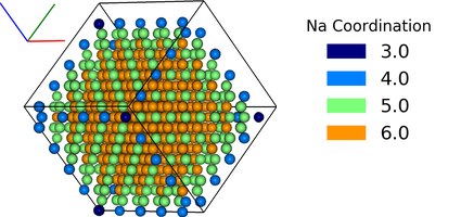
Atomic Coordination
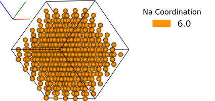
The two examples below show computation of the coordination of Na, w.r.t Cl, in a simple NaCl crystal (which should be 6). The first does not include a consideration of the repeating boundary conditions, and so outer atoms have a lower coordination number. But the latter computation provides a method which takes this into consideration, by repeating the Cl lattice in each direction before computation.
data = ipymd.data_input.crystal.Crystal()
data.setup_data(
    [[0.0, 0.0, 0.0], [0.5, 0.5, 0.5]], ['Na', 'Cl'],
    225, cellpar=[5.4, 5.4, 5.4, 90, 90, 90],
    repetitions=[5, 5, 5])
df = data.get_atom_data()
meta = data.get_meta_data()

df = ipymd.atom_analysis.nearest_neighbour.coordination_bytype(df, 'Na','Cl')

new_df = manipulate_atoms(df,meta)
new_df.filter_variables('Na')
new_df.color_by_variable('coord_Na_Cl',minv=3,maxv=7)

vis = ipymd.visualise_sim.Visualise_Sim()
vis.add_axes(offset=(0,-0.3))
vis.add_box(*meta[['a','b','c','origin']])
vis.add_atoms(new_df.df)

img = vis.get_image(xrot=45,yrot=45)

img2 = ipymd.plotting.create_legend_image(new_df.df.coord_Na_Cl,new_df.df.color, title='Na Coordination',size=150,colbytes=True)

vis.visualise([img,img2],columns=2)
data = ipymd.data_input.crystal.Crystal()
data.setup_data(
    [[0.0, 0.0, 0.0], [0.5, 0.5, 0.5]], ['Na', 'Cl'],
    225, cellpar=[5.4, 5.4, 5.4, 90, 90, 90],
    repetitions=[5, 5, 5])
df = data.get_atom_data()
meta = data.get_meta_data()

df = ipymd.atom_analysis.nearest_neighbour.coordination_bytype(
    df, 'Na','Cl',repeat_meta=meta)

new_df = manipulate_atoms(df)
new_df.filter_variables('Na')
new_df.color_by_variable('coord_Na_Cl',minv=3,maxv=7)

vis = ipymd.visualise_sim.Visualise_Sim()
vis.add_box(*meta[['a','b','c','origin']])
vis.add_axes(offset=(0,-0.3))
vis.add_atoms(new_df.df)

img = vis.get_image(xrot=45,yrot=45)

img2 = ipymd.plotting.create_legend_image(new_df.df.coord_Na_Cl,new_df.df.color, title='Na Coordination',size=150,colbytes=True)

vis.visualise([img,img2],columns=2)
Atomic Structure Comparison
compare_to_lattice takes each atomic coordinate in df1 and computes
the distance to the nearest atom (i.e. lattice site) in df2:
import numpy as np
data1 = ipymd.data_input.crystal.Crystal()
data1.setup_data(
    [[0.0, 0.0, 0.0], [0.5, 0.5, 0.5]], ['Na', 'Cl'],
    225, cellpar=[5.4, 5.4, 5.4, 90, 90, 90],
    repetitions=[5, 5, 5])
df1 = data1.get_atom_data()

print(('Average distance to nearest atom (identical)',
       np.mean(ipymd.atom_analysis.nearest_neighbour.compare_to_lattice(df1,df1))))

data2 = ipymd.data_input.crystal.Crystal()
data2.setup_data(
    [[0.0, 0.0, 0.0], [0.5, 0.5, 0.5]], ['Na', 'Cl'],
    225, cellpar=[5.41, 5.4, 5.4, 90, 90, 90],
    repetitions=[5, 5, 5])
df2 = data2.get_atom_data()

print(('Average distance to nearest atom (different)',
       np.mean(ipymd.atom_analysis.nearest_neighbour.compare_to_lattice(df1,df2))))
('Average distance to nearest atom (identical)', 0.0)
('Average distance to nearest atom (different)', 0.022499999999999343)
Common Neighbour Analysis (CNA)
CNA (Honeycutt and Andersen, J. Phys. Chem. 91, 4950) is an algorithm to compute a signature for pairs of atoms, which is designed to characterize the local structural environment. Typically, CNA is used as an effective filtering method to classify atoms in crystalline systems (Faken and Jonsson, Comput. Mater. Sci. 2, 279, with the goal to get a precise understanding of which atoms are associated with which phases, and which are associated with defects.
Common signatures for nearest neighbours are:
- FCC = 12 x 4,2,1
- HCP = 6 x 4,2,1 & 6 x 4,2,2
- BCC = 6 x 6,6,6 & 8 x 4,4,4
- Diamond = 12 x 5,4,3 & 4 x 6,6,3
which are tested below:
data = ipymd.data_input.crystal.Crystal()
data.setup_data(
    [[0.0, 0.0, 0.0]], ['Al'],
    225, cellpar=[4.05, 4.05, 4.05, 90, 90, 90],
    repetitions=[5, 5, 5])
fcc_meta = data.get_meta_data()
fcc_df = data.get_atom_data()

data = ipymd.data_input.crystal.Crystal()
data.setup_data(
    [[0.33333,0.66667,0.25000]], ['Mg'],
    194, cellpar=[3.21, 3.21, 5.21, 90, 90, 120],
    repetitions=[5,5,5])
hcp_meta = data.get_meta_data()
hcp_df = data.get_atom_data()

data = ipymd.data_input.crystal.Crystal()
data.setup_data(
    [[0,0,0]], ['Fe'],
    229, cellpar=[2.866, 2.866, 2.866, 90, 90, 90],
    repetitions=[5,5,5])
bcc_meta = data.get_meta_data()
bcc_df = data.get_atom_data()

data = ipymd.data_input.crystal.Crystal()
data.setup_data(
    [[0,0,0]], ['C'],
    227, cellpar=[3.57, 3.57, 3.57, 90, 90, 90],
    repetitions=[2,2,2])
diamond_meta = data.get_meta_data()
diamond_df = data.get_atom_data()
print(ipymd.atom_analysis.nearest_neighbour.cna_sum(fcc_df,repeat_meta=fcc_meta))
print(ipymd.atom_analysis.nearest_neighbour.cna_sum(hcp_df,repeat_meta=hcp_meta))
print(ipymd.atom_analysis.nearest_neighbour.cna_sum(bcc_df,repeat_meta=bcc_meta))
print(ipymd.atom_analysis.nearest_neighbour.cna_sum(diamond_df,upper_bound=10,max_neighbours=16,
                                                    repeat_meta=diamond_meta))
Counter({'4,2,1': 6000})
Counter({'4,2,2': 1500, '4,2,1': 1500})
Counter({'6,6,6': 2000, '4,4,4': 1500})
Counter({'5,4,3': 768, '6,6,3': 256})
For each atom, the CNA for each nearest-neighbour can be output:
ipymd.atom_analysis.nearest_neighbour.common_neighbour_analysis(hcp_df,repeat_meta=hcp_meta).head(5)
| id | type | x | y | z | transparency | color | radius | cna | |
|---|---|---|---|---|---|---|---|---|---|
| 0 | 1 | Mg | -0.000016 | 1.853304 | 1.3025 | 1.0 | light_salmon | 1.0 | {u'4,2,2': 6, u'4,2,1': 6} |
| 1 | 2 | Mg | 1.605016 | 0.926638 | 3.9075 | 1.0 | light_salmon | 1.0 | {u'4,2,2': 6, u'4,2,1': 6} |
| 2 | 3 | Mg | -0.000016 | 1.853304 | 6.5125 | 1.0 | light_salmon | 1.0 | {u'4,2,2': 6, u'4,2,1': 6} |
| 3 | 4 | Mg | 1.605016 | 0.926638 | 9.1175 | 1.0 | light_salmon | 1.0 | {u'4,2,2': 6, u'4,2,1': 6} |
| 4 | 5 | Mg | -0.000016 | 1.853304 | 11.7225 | 1.0 | light_salmon | 1.0 | {u'4,2,2': 6, u'4,2,1': 6} |
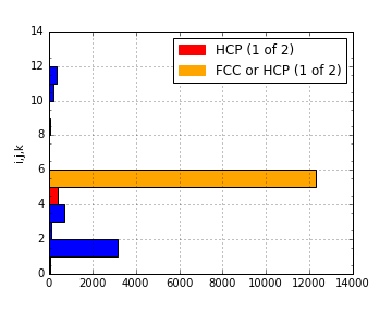
This can be used to produce a plot identifying likely structure of an unknown structure:
lammps_path = ipymd.get_data_path('thermalized_troilite.dump')
data = ipymd.data_input.lammps.LAMMPS_Output()
data.setup_data(lammps_path)
df = data.get_atom_data()
df = df[df.type==1]
plot = ipymd.atom_analysis.nearest_neighbour.cna_plot(df,repeat_meta=data.get_meta_data())
plot.display_plot()
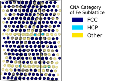
A visualisation of the probable local character of each atom can also be
created. Note the accuracy parameter in the cna_categories method
allows for more robust fitting to the ideal signatures:
lammps_path = ipymd.get_data_path('thermalized_troilite.dump')
data = ipymd.data_input.lammps.LAMMPS_Output()
data.setup_data(lammps_path)
df = data.get_atom_data()
meta = data.get_meta_data()
df = df[df.type==1]
df = ipymd.atom_analysis.nearest_neighbour.cna_categories(
    df,repeat_meta=meta,accuracy=0.7)
manip = ipymd.atom_manipulation.Atom_Manipulation(df)
manip.color_by_categories('cna')
#manip.apply_colormap({'Other':'blue','FCC':'green','HCP':'red'}, type_col='cna')
manip.change_type_variable('Other','transparency',0.5,type_col='cna')
atom_df = manip.df

vis = ipymd.visualise_sim.Visualise_Sim()
vis.add_box(*meta[['a','b','c','origin']])
vis.add_atoms(atom_df)

img = vis.get_image(xrot=90)

img2 = ipymd.plotting.create_legend_image(atom_df.cna,atom_df.color,
                title='CNA Category\nof Fe Sublattice',size=150,colbytes=True)

vis.visualise([img,img2],columns=2)
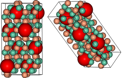
Vacany Identification
The vacancy_identification method finds grid sites with no atoms
within a specified distance:
cif_path = ipymd.get_data_path('pyr_4C_monoclinic.cif')
data = ipymd.data_input.cif.CIF()
data.setup_data(cif_path)
cif4c_df, cif4c_meta = data.get_atom_data(), data.get_meta_data()
vac_df = ipymd.atom_analysis.nearest_neighbour.vacancy_identification(cif4c_df,0.2,2.3,cif4c_meta,
                                         radius=2.3,remove_dups=True)
vis = ipymd.visualise_sim.Visualise_Sim()
vis.add_atoms(vac_df)
vis.add_box(*cif4c_meta[['a','b','c','origin']])
vis.add_atoms(cif4c_df)
vis.visualise([vis.get_image(xrot=90,yrot=10),
               vis.get_image(xrot=45,yrot=45)],columns=2)
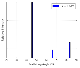
XRD Spectrum Prediction
This is an implementation of the virtual x-ray diffraction pattern algorithm, from http://http://dx.doi.org/10.1007/s11837-013-0829-3.
data = ipymd.data_input.crystal.Crystal()
data.setup_data(
    [[0,0,0]], ['Fe'],
    229, cellpar=[2.866, 2.866, 2.866, 90, 90, 90],
    repetitions=[5,5,5])

meta = data.get_meta_data()
atoms_df = data.get_atom_data()

wlambda = 1.542 # Angstrom (Cu K-alpha)
thetas, Is = ipymd.atom_analysis.spectral.compute_xrd(atoms_df,meta,wlambda)
plot = ipymd.atom_analysis.spectral.plot_xrd_hist(thetas,Is,wlambda=wlambda,barwidth=1)
plot.axes.set_xlim(20,90)
plot.display_plot(True)
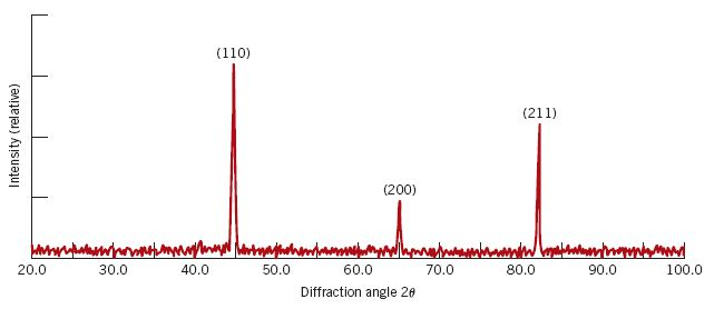
The predicted spectrum peaks (for alpha-Fe) shows good correlation with experimentally derived data:
from IPython.display import Image
exp_path = ipymd.get_data_path('xrd_fe_bcc_Cu_kalpha.png',
                          module=ipymd.atom_analysis)
Image(exp_path,width=380)
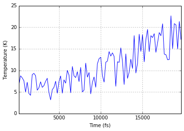
System Analysis
Within the LAMMPS_Output class there is also the option to read in a
systems data file, with a log of global variables for each simulation
timestep.
data = ipymd.data_input.lammps.LAMMPS_Output()
sys_path = ipymd.get_data_path('system.dump')
data.setup_data(sys_path=sys_path)
sys_data = data.get_meta_data_all()
sys_data.head()
| time | natoms | a | b | vol | press | temp | peng | keng | teng | enth | |
|---|---|---|---|---|---|---|---|---|---|---|---|
| config | |||||||||||
| 2 | 200 | 5880 | 3.997601 | 3.997601 | 106784.302378 | 2568.163297 | 6.616167 | -576911.132565 | 115.942920 | -576795.189644 | -572795.687453 |
| 3 | 400 | 5880 | 3.993996 | 3.993997 | 106591.809864 | 1560.503603 | 8.739034 | -576962.187377 | 153.144425 | -576809.042952 | -574383.189834 |
| 4 | 600 | 5880 | 3.989881 | 3.989882 | 106372.285789 | 364.540620 | 8.262727 | -576965.242403 | 144.797535 | -576820.444868 | -576254.921821 |
| 5 | 800 | 5880 | 3.986465 | 3.986465 | 106190.203677 | -586.959616 | 7.597382 | -576960.911674 | 133.137903 | -576827.773772 | -577736.783571 |
| 6 | 1000 | 5880 | 3.988207 | 3.988208 | 106283.055838 | 128.391396 | 4.990469 | -576921.379605 | 87.453896 | -576833.925708 | -576634.915276 |
ax = sys_data.plot('time','temp',legend=False)
ax.set_xlabel('Time (fs)')
ax.set_ylabel('Temperature (K)');
ax.grid()
Plotting
Plotting is handled by the Plotter class, which is mainly a useful
wrapper around matplotlib.
df = pd.DataFrame(
[[2,3,4,1,[0, 0, 255],1],
[1,3,3,1,'orange',1],
[4,3,1,1,'blue',1]],
columns=['x','y','z','radius','color','transparency'])
vis = ipymd.visualise_sim.Visualise_Sim()
vis.add_atoms(df)
vis.add_axes(length=0.2, offset=(-0.3,0))
vis.add_box([5,0,0],[0,5,0],[0,0,5])
vis.add_plane([[5,0,0],[0,5,2]],alpha=0.3)
vis.add_hexagon([[1,0,0],[0,0,.5]],[0,0,2],color='green')
img_ex1 = vis.get_image(xrot=45, yrot=45)
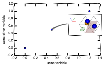
with ipymd.plotting.style('xkcd'):
plot = ipymd.plotting.Plotter(figsize=(5,3))
plot.axes.scatter([0,0.5,1.2],[0,0.5,1],s=30)
plot.axes.set_xlabel('some variable')
plot.axes.set_ylabel('some other variable')
plot.add_image_annotation(img_ex1,(230,100),(0.5,0.5),zoom=0.5)
plot.display_plot(tight_layout=True)
Matplotlib also has an animation capability:
import numpy as np
x_iter = [np.linspace(0, 2, 1000) for i in range(100)]
def y_iter(x_iter):
    for i,x in enumerate(x_iter):
        yield np.sin(2 * np.pi * (x - 0.01 * i))

with ipymd.plotting.style('ggplot'):
    line_anim = ipymd.plotting.animation_line(x_iter,y_iter(x_iter),
                                              xlim=(0,2),ylim=(-2,2),incl_controls=False)
line_anim
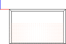
Recent IPython Notebook version have brought powerful new interactive features, such as Javascript widgets:
One could imagine using this feature to overlay time-dependant field information on to 2D visualiations of atomic configurations:
# visualise atoms
df = pd.DataFrame(
        [[2,3,4,1,'gray',0.6],
         [1,3,3,1,'gray',0.6],
         [4,3,1,1,'gray',0.6]],
        columns=['x','y','z','radius','color','transparency'])
vis = ipymd.visualise_sim.Visualise_Sim()
vis.add_atoms(df,illustrate=True)
img1 = vis.get_image(size=400,quality=5,xrot=90)

plot = ipymd.plotting.Plotter()
plot.add_image(img1,width=2,height=2,origin=(-1,-1))

# setup contour iterators
import numpy as np
from itertools import izip
from matplotlib.mlab import bivariate_normal

x_iter = [np.linspace(-1, 1, 1000) for i in range(100)]
y_iter = [np.linspace(-1, 1, 1000) for i in range(100)]
def z_iter(x_iter,y_iter):
    for i,(x,y) in enumerate(izip(x_iter,y_iter)):
        X, Y = np.meshgrid(x, y)
        yield bivariate_normal(X, Y, 0.005*(i+1), 0.005*(i+1),0.5,0.5)

# create contour visualisation
with ipymd.plotting.style('ggplot'):
    c_anim = ipymd.plotting.animation_contourf(x_iter,y_iter,z_iter(x_iter,y_iter),
                                      xlim=(-1,1),ylim=(-1,1),
                                      cmap='PuBu_r',alpha=0.5,plot=plot)
c_anim