ipymd.atom_analysis package

Subpackages

Submodules

ipymd.atom_analysis.basic module

Created on Thu Jul 14 14:06:40 2016

@author: cjs14

functions to calculate basic properties of the atoms

ipymd.atom_analysis.basic.density_bb(atoms_df, vectors=[[1, 0, 0], [0, 1, 0], [0, 0, 1]])

calculate density of the bounding box (assuming all atoms are inside)

ipymd.atom_analysis.basic.lattparams_bb(vectors=[[1, 0, 0], [0, 1, 0], [0, 0, 1]], rounded=None, cells=(1, 1, 1))

calculate unit cell parameters of the bounding box

rounded : int

the number of decimal places to return

cells : (int,int,int)

how many unit cells the vectors represent in each direction

Returns: Return type:a, b, c, alpha, beta, gamma (in degrees)

ipymd.atom_analysis.basic.volume_bb(vectors=[[1, 0, 0], [0, 1, 0], [0, 0, 1]], rounded=None, cells=(1, 1, 1))

calculate volume of the bounding box

rounded : int

the number of decimal places to return

cells : (int,int,int)

how many unit cells the vectors represent in each direction

Returns:volume Return type:float

ipymd.atom_analysis.basic.volume_points(atoms_df)

calculate volume of the shape encompasing all atom coordinates

ipymd.atom_analysis.nearest_neighbour module

Created on Thu Jul 14 14:05:09 2016

@author: cjs14

functions based on nearest neighbour calculations

ipymd.atom_analysis.nearest_neighbour.bond_lengths(atoms_df, coord_type, lattice_type, max_dist=4, max_coord=16, repeat_meta=None, rounded=2, min_dist=0.01, leafsize=100)

calculate the unique bond lengths atoms in coords_atoms, w.r.t lattice_atoms

atoms_df : pandas.Dataframe

all atoms

coord_type : string

atoms to calcualte coordination of

lattice_type : string

atoms to act as lattice for coordination

max_dist : float

maximum distance for coordination consideration

max_coord : float

maximum possible coordination number

repeat_meta : pandas.Series

include consideration of repeating boundary idenfined by a,b,c in the meta data

min_dist : float

lattice points within this distance of the atom will be ignored (assumed self-interaction)

leafsize : int

points at which the algorithm switches to brute-force (kdtree specific)

Returns:distances – list of unique distances Return type:set

ipymd.atom_analysis.nearest_neighbour.cna_categories(atoms_df, accuracy=1.0, upper_bound=4, max_neighbours=24, repeat_meta=None, leafsize=100, ipython_progress=False)

compute summed atomic environments of each atom in atoms_df

Based on Faken, Daniel and Jónsson, Hannes, ‘Systematic analysis of local atomic structure combined with 3D computer graphics’, March 1994, DOI: 10.1016/0927-0256(94)90109-0

signatures: - FCC = 12 x 4,2,1 - HCP = 6 x 4,2,1 & 6 x 4,2,2 - BCC = 6 x 6,6,6 & 8 x 4,4,4 - Diamond = 12 x 5,4,3 & 4 x 6,6,3 - Icosahedral = 12 x 5,5,5

Parameters:

• accuracy (float) – 0 to 1 how accurate to fit to signature
• repeat_meta (pandas.Series) – include consideration of repeating boundary idenfined by a,b,c in the meta data
• ipython_progress (bool) – print progress to IPython Notebook

Returns:

df – copy of atoms_df with new column named cna

Return type:

pandas.Dataframe

ipymd.atom_analysis.nearest_neighbour.cna_plot(atoms_df, upper_bound=4, max_neighbours=24, repeat_meta=None, leafsize=100, barwidth=1, ipython_progress=False)

compute summed atomic environments of each atom in atoms_df

Based on Faken, Daniel and Jónsson, Hannes, ‘Systematic analysis of local atomic structure combined with 3D computer graphics’, March 1994, DOI: 10.1016/0927-0256(94)90109-0

common signatures: - FCC = 12 x 4,2,1 - HCP = 6 x 4,2,1 & 6 x 4,2,2 - BCC = 6 x 6,6,6 & 8 x 4,4,4 - Diamond = 12 x 5,4,3 & 4 x 6,6,3 - Icosahedral = 12 x 5,5,5

Parameters:

• repeat_meta (pandas.Series) – include consideration of repeating boundary idenfined by a,b,c in the meta data
• ipython_progress (bool) – print progress to IPython Notebook

Returns:

plot – a matplotlib plot

Return type:

matplotlib.pyplot

ipymd.atom_analysis.nearest_neighbour.cna_sum(atoms_df, upper_bound=4, max_neighbours=24, repeat_meta=None, leafsize=100, ipython_progress=False)

compute summed atomic environments of each atom in atoms_df

Based on Faken, Daniel and Jónsson, Hannes, ‘Systematic analysis of local atomic structure combined with 3D computer graphics’, March 1994, DOI: 10.1016/0927-0256(94)90109-0

common signatures: - FCC = 12 x 4,2,1 - HCP = 6 x 4,2,1 & 6 x 4,2,2 - BCC = 6 x 6,6,6 & 8 x 4,4,4 - Diamond = 12 x 5,4,3 & 4 x 6,6,3 - Icosahedral = 12 x 5,5,5

Parameters:

• repeat_meta (pandas.Series) – include consideration of repeating boundary idenfined by a,b,c in the meta data
• ipython_progress (bool) – print progress to IPython Notebook

Returns:

counter – a counter of cna signatures

Return type:

Counter

ipymd.atom_analysis.nearest_neighbour.common_neighbour_analysis(atoms_df, upper_bound=4, max_neighbours=24, repeat_meta=None, leafsize=100, ipython_progress=False)

compute atomic environment of each atom in atoms_df

Based on Faken, Daniel and Jónsson, Hannes, ‘Systematic analysis of local atomic structure combined with 3D computer graphics’, March 1994, DOI: 10.1016/0927-0256(94)90109-0

ideally: - FCC = 12 x 4,2,1 - HCP = 6 x 4,2,1 & 6 x 4,2,2 - BCC = 6 x 6,6,6 & 8 x 4,4,4 - icosahedral = 12 x 5,5,5

repeat_meta : pandas.Series

include consideration of repeating boundary idenfined by a,b,c in the meta data

ipython_progress : bool

print progress to IPython Notebook

Returns:df – copy of atoms_df with new column named cna Return type:pandas.Dataframe

ipymd.atom_analysis.nearest_neighbour.compare_to_lattice(atoms_df, lattice_atoms_df, max_dist=10, leafsize=100)

calculate the minimum distance of each atom in atoms_df from a lattice point in lattice_atoms_df

atoms_df : pandas.Dataframe

atoms to calculate for

lattice_atoms_df : pandas.Dataframe

atoms to act as lattice points

max_dist : float

maximum distance for consideration in computation

leafsize : int

points at which the algorithm switches to brute-force (kdtree specific)

Returns:distances – list of distances to nearest atom in lattice Return type:list

ipymd.atom_analysis.nearest_neighbour.coordination(coord_atoms_df, lattice_atoms_df, max_dist=4, max_coord=16, repeat_meta=None, min_dist=0.01, leafsize=100)

calculate the coordination number of each atom in coords_atoms, w.r.t lattice_atoms

coords_atoms_df : pandas.Dataframe

atoms to calcualte coordination of

lattice_atoms_df : pandas.Dataframe

atoms to act as lattice for coordination

max_dist : float

maximum distance for coordination consideration

max_coord : float

maximum possible coordination number

repeat_meta : pandas.Series

include consideration of repeating boundary idenfined by a,b,c in the meta data

min_dist : float

lattice points within this distance of the atom will be ignored (assumed self-interaction)

leafsize : int

points at which the algorithm switches to brute-force (kdtree specific)

Returns:coords – list of coordination numbers Return type:list

ipymd.atom_analysis.nearest_neighbour.coordination_bytype(atoms_df, coord_type, lattice_type, max_dist=4, max_coord=16, repeat_meta=None, min_dist=0.01, leafsize=100)

returns dataframe with additional column for the coordination number of each atom of coord type, w.r.t lattice_type atoms

effectively an extension of calc_df_coordination

atoms_df : pandas.Dataframe

all atoms

coord_type : string

atoms to calcualte coordination of

lattice_type : string

atoms to act as lattice for coordination

max_dist : float

maximum distance for coordination consideration

max_coord : float

maximum possible coordination number

repeat_meta : pandas.Series

include consideration of repeating boundary idenfined by a,b,c in the meta data

min_dist : float

lattice points within this distance of the atom will be ignored (assumed self-interaction)

leafsize : int

points at which the algorithm switches to brute-force (kdtree specific)

Returns:df – copy of atoms_df with new column named coord_{coord_type}_{lattice_type} Return type:pandas.Dataframe

ipymd.atom_analysis.nearest_neighbour.guess_bonds(atoms_df, covalent_radii=None, threshold=0.1, max_length=5.0, radius=0.1, transparency=1.0, color=None)

guess bonds between atoms, based on approximate covalent radii

Parameters:

• atoms_df (pandas.Dataframe) – all atoms, requires colums [‘x’,’y’,’z’,’type’, ‘color’]
• covalent_radii (dict or None) – a dict of covalent radii for each atom type, if None then taken from ipymd.shared.atom_data
• threshold (float) – include bonds with distance +/- threshold of guessed bond length (Angstrom)
• max_length (float) – maximum bond length to include (Angstrom)
• radius (float) – radius of displayed bond cylinder (Angstrom)
• transparency (float) – transparency of displayed bond cylinder
• color (str or tuple) – color of displayed bond cylinder, if None then colored by atom color

Returns:

bonds_df – a dataframe with start/end indexes relating to atoms in atoms_df

Return type:

pandas.Dataframe

ipymd.atom_analysis.nearest_neighbour.vacancy_identification(atoms_df, res=0.2, nn_dist=2.0, repeat_meta=None, remove_dups=True, color='red', transparency=1.0, radius=1, type_name='Vac', leafsize=100, n_jobs=1, ipython_progress=False)

identify vacancies

atoms_df : pandas.Dataframe

atoms to calculate for

res : float

resolution of vacancy identification, i.e. spacing of reference lattice

nn_dist : float

maximum nearest-neighbour distance considered as a vacancy

repeat_meta : pandas.Series

include consideration of repeating boundary idenfined by a,b,c in the meta data

remove_dups : bool

only keep one vacancy site within the nearest-neighbour distance

leafsize : int

points at which the algorithm switches to brute-force (kdtree specific)

n_jobs : int, optional

Number of jobs to schedule for parallel processing. If -1 is given all processors are used.

ipython_progress : bool

print progress to IPython Notebook

Returns:vac_df – new atom dataframe of vacancy sites as atoms Return type:pandas.DataFrame

ipymd.atom_analysis.spectral module

Created on Tue Jul 12 20:18:04 2016

Derived from: LAMMPS - Large-scale Atomic/Molecular Massively Parallel Simulator http://lammps.sandia.gov, Sandia National Laboratories Steve Plimpton, sjplimp@sandia.gov Copyright (2003) Sandia Corporation. Under the terms of Contract DE-AC04-94AL85000 with Sandia Corporation, the U.S. Government retains certain rights in this software. This software is distributed under the GNU General Public License. https://github.com/lammps/lammps/tree/lammps-icms/src/USER-DIFFRACTION

This package contains the commands neeed to calculate x-ray and electron diffraction intensities based on kinematic diffraction theory. Detailed discription of the computation can be found in the following works:

Coleman, S.P., Spearot, D.E., Capolungo, L. (2013) Virtual diffraction analysis of Ni [010] symmetric tilt grain boundaries, Modelling and Simulation in Materials Science and Engineering, 21 055020. doi:10.1088/0965-0393/21/5/055020

Coleman, S.P., Sichani, M.M., Spearot, D.E. (2014) A computational algorithm to produce virtual x-ray and electron diffraction patterns from atomistic simulations, JOM, 66 (3), 408-416. doi:10.1007/s11837-013-0829-3

Coleman, S.P., Pamidighantam, S. Van Moer, M., Wang, Y., Koesterke, L. Spearot D.E (2014) Performance improvement and workflow development of virtual diffraction calculations, XSEDE14, doi:10.1145/2616498.2616552

@author: chris sewell

ipymd.atom_analysis.spectral.get_sf_coeffs()

ipymd.atom_analysis.spectral.xrd_compute(atoms_df, meta_data, wlambda, min2theta=1.0, max2theta=179.0, lp=True, rspace=[1, 1, 1], manual=False, periodic=[True, True, True])

Compute predicted x-ray diffraction intensities for a given wavelength

atoms_df : pandas.DataFrame

a dataframe of info for each atom, including columns; x,y,z,type

meta_data : pandas.Series

data of a,b,c crystal vectors (as tuples, e.g. meta_data.a = (0,0,1))

wlambda : float

radiation wavelength (length units) typical values are Cu Ka = 1.54, Mo Ka = 0.71 Angstroms

min2theta : float

minimum 2 theta range to explore (degrees)

max2theta : float

maximum 2 theta range to explore (degrees)

lp : bool

switch to apply Lorentz-polarization factor

use_triclinic : bool

use_triclinic

rspace : list of floats

parameters to adjust the spacing of the reciprocal lattice nodes in the h, k, and l directions respectively

manual : bool

use manual spacing of reciprocal lattice points based on the values of the c parameters (good for comparing diffraction results from multiple simulations, but small c required).

periodic : list of bools

whether periodic boundary in the h, k, and l directions respectively

Returns:df – theta (in degrees), I, h, k and l for each k-point Return type:pandas.DataFrame

Notes

This is an implementation of the virtual x-ray diffraction pattern algorithm by Coleman et al. [ref1]

The algorithm proceeds in the following manner:

1. Define a crystal structure by position (x,y,z) and atom/ion type.
2. Define the x-ray wavelength to use
3. Compute the full reciprocal lattice mesh
4. Filter reciprocal lattice points by those in the Eswald’s sphere
5. Compute the structure factor at each reciprocal lattice point, for each atom type
6. Compute the x-ray diffraction intensity at each reciprocal lattice point
7. Group and sum intensities by angle

reciprocal points of the lattice are computed such that:

\[\mathbf{K} = {m_{1}}\cdot \mathbf{b}_{1}+{m_{2}}\cdot \mathbf{b}_{2}+{m_{3}}\cdot \mathbf{b}_{3}\]

where,

\[\begin{split}\begin{aligned} \mathbf {b_{1}} &= {\frac {\mathbf {a_{2}} \times \mathbf {a_{3}} }{\mathbf {a_{1}} \cdot (\mathbf {a_{2}} \times \mathbf {a_{3}} )}}\\ \mathbf {b_{2}} &= {\frac {\mathbf {a_{3}} \times \mathbf {a_{1}} }{\mathbf {a_{2}} \cdot (\mathbf {a_{3}} \times \mathbf {a_{1}} )}}\\ \mathbf {b_{3}} &= {\frac {\mathbf {a_{1}} \times \mathbf {a_{2}} }{\mathbf {a_{3}} \cdot (\mathbf {a_{1}} \times \mathbf {a_{2}} )}} \end{aligned}\end{split}\]

The reciprocal k-point modulii of the x-ray is calculated from Bragg’s law:

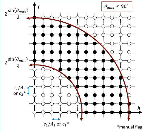
\[\left| {\mathbf{K}_{\lambda}} \right| = \frac{1}{{d_{\text{hkl}} }} = \frac{2\sin \left( \theta \right)}{\lambda }\]

This is used to construct an Eswald’s sphere, and only reciprocal lattice ponts within are retained, as illustrated:

The atomic scattering factors, fj, accounts for the reduction in diffraction intensity due to Compton scattering, with coefficients based on the electron density around the atomic nuclei.

\[f_j \left(\frac{\sin \theta}{\lambda}\right) = \left[ \sum\limits^4_i a_i \exp \left( -b_i \frac{\sin^2 \theta}{\lambda^2} \right)\right] + c = \left[ \sum\limits^4_i a_i \exp \left( -b_i \left(\frac{\left| {\mathbf{K}} \right|}{2}\right)^2 \right)\right] + c\]

The relative diffraction intensity from x-rays is computed at each reciprocal lattice point through:

\[I_x(\mathbf{K}) = Lp(\theta) \frac{F(\mathbf{K})F^*(\mathbf{K})}{N}\]

such that:

\[F ({\mathbf{K}} )= \sum\limits_{j = 1}^{N} {f_{j}.e^{\left( {2\pi i \, {\mathbf{K}} \cdot {\mathbf{r}}_{j} } \right)}} = \sum\limits_{j = 1}^{N} {f_j.\left[ \cos \left( 2\pi \mathbf{K} \cdot \mathbf{r}_j \right) + i \sin \left( 2\pi \mathbf{K} \cdot \mathbf{r}_j \right) \right]}\]

and the Lorentz-polarization factor is:

\[Lp(\theta) = \frac{1+\cos^2 (2\theta)}{\cos(\theta)\sin^2(\theta)}\]

References

[ref1]

1.Coleman, S. P., Sichani, M. M. & Spearot, D. E. A Computational Algorithm to Produce Virtual X-ray and Electron Diffraction Patterns from Atomistic Simulations. JOM 66, 408–416 (2014).

ipymd.atom_analysis.spectral.xrd_group_i(df, tstep=None, sym_equiv_hkl='none')

group xrd intensities by theta

Parameters:

• df (pandas.DataFrame) – containing columns; [‘theta’,’I’] and optional [‘h’,’k’,’l’]
• tstep (None or float) – if not None, group thetas within ranges i to i+tstep
• sym_equiv_hkl (str) – group hkl by symmetry-equivalent refelections; [‘none’,’mmm’,’m-3m’]

Returns:

df

Return type:

pandas.DataFrame

Notes

if grouping by theta step, then the theta value for each group will be the intensity weighted average

Crystal System | Laue Class | Symmetry-Equivalent Reflections | Multiplicity ————– | ———- | ——————————- | ———— Triclinic | -1 | hkl ≡ -h-k-l | 2 Monoclinic | 2/m | hkl ≡ -hk-l ≡ -h-k-l ≡ h-kl | 4 Orthorhombic | mmm | hkl ≡ h-k-l ≡ -hk-l ≡ -h-kl ≡ -h-k-l ≡ -hkl ≡ h-kl ≡ hk-l | 8 Tetragonal | 4/m | hkl ≡ -khl ≡ -h-kl ≡ k-hl ≡ -h-k-l ≡ k-h-l ≡ hk-l ≡ -kh-l | 8

4/mmm | hkl ≡ -khl ≡ -h-kl ≡ k-hl ≡ -h-k-l ≡ k-h-l ≡ hk-l ≡ -kh-l |

| ≡ khl ≡ -hkl ≡ -k-hl ≡ h-kl ≡ -k-h-l ≡ h-k-l ≡ kh-l ≡ -hk-l | 16

Cubic | m-3 | hkl ≡ -hkl ≡ h-kl ≡ hk-l ≡ -h-k-l ≡ h-k-l ≡ -hk-l ≡ -h-kl |

| ≡ klh ≡ -klh ≡ k-lh ≡ kl-h ≡ -k-l-h ≡ k-l-h ≡ -kl-h ≡ -k-lh |

| ≡ lhk ≡ -lhk ≡ l-hk ≡ lh-k ≡ -l-h-k ≡ l-h-k ≡ -lh-k ≡ -l-hk | 24

m-3m | hkl ≡ -hkl ≡ h-kl ≡ hk-l ≡ -h-k-l ≡ h-k-l ≡ -hk-l ≡ -h-kl |

| ≡ klh ≡ -klh ≡ k-lh ≡ kl-h ≡ -k-l-h ≡ k-l-h ≡ -kl-h ≡ -k-lh |

| ≡ lhk ≡ -lhk ≡ l-hk ≡ lh-k ≡ -l-h-k ≡ l-h-k ≡ -lh-k ≡ -l-hk |

| ≡ khl ≡ -khl ≡ k-hl ≡ kh-l ≡ -k-h-l ≡ k-h-l ≡ -kh-l ≡ -k-hl |

| ≡ lkh ≡ -lkh ≡ l-kh ≡ lk-h ≡ -l-k-h ≡ l-k-h ≡ -lk-h ≡ -l-kh |

| ≡ hlk ≡ -hlk ≡ h-lk ≡ hl-k ≡ -h-l-k ≡ h-l-k ≡ -hl-k ≡ -h-lk | 48

ipymd.atom_analysis.spectral.xrd_plot(df, icol='I_norm', imin=0.01, barwidth=1.0, hkl_num=0, hkl_trange=[0.0, 180.0], incl_multi=False, label_inline=True, label_trange=[0.0, 180.0], ax=None, **kwargs)

create plot of xrd pattern

df : pd.DataFrame

containing columns [‘theta’,icol] and optional [‘hkl’,’multiplicity’]

icol : str

column name for intensity data

imin : float

minimum intensity to display

barwidth : float or None

if None then the barwidth will be the bin width

hkl_num : int

number of k-point values to label

hkl_trange : [float,float]

theta range within which to label peaks with k-point values

label_inline : bool

place k-point labels inline or at top of plot

label_trange : [float,float]

if not inline, theta range within which to fit k-point labels

incl_multi : bool

add multiplicity to k-point label

kwargs : optional

additional arguments for bar plot (e.g. label, color, alpha)

Returns:plot – a plot object Return type:ipymd.plotting.Plotting

Module contents